| Like
copper wire, fiber optic cable is available in many physical
variations. There are single and multiple conductor constructions,
aerial and direct burial styles, plenum and riser cables and
even ultra-rugged military type tactical cables that will withstand severe
mechanical abuse. Which cable one chooses is, of course, dependent
upon the application.
Regardless of the
final outer construction however, all fiber optic cable contains one or
more optical fibers. These fibers are protected by an internal
construction that is unique to fiber optic cable. The two most
common protection schemes in use today are to enclose the tiny fiber in a
loose fitting tube or to coat the fiber with a tight fitting buffer
coating.
In the loose tube
method the fiber is enclosed in a plastic buffer-tube that is larger in
inner diameter than the outer diameter of the fiber itself. This
tube is sometimes filled with a silicone gel to prevent the buildup of
moisture as well. Since the fiber is basically free to float
within the tube, mechanical forces acting on the outside of the cable do
not usually reach the fiber.
Cable containing loose buffer-tube fiber
is generally very tolerant of axial forces of the type encountered when
pulling through conduits or where constant mechanical stress is present
such as cables employed for aerial use. Since the fiber is not under
any significant strain, loose buffer-tube cables exhibit low optical
attenuation losses.
In the tight buffer
construction, a thick coating of a plastic-type material is applied
directly to the outside of the fiber itself. This results in a
smaller overall diameter of the entire cable and one that is more
resistant to crushing or overall impact- type forces. Because the
fiber is not free to float however, tensile strength is not as
great. Tight buffer cable is normally lighter in weight and more
flexible than loose-tube cable and is usually employed for less severe
applications such as within a building or to interconnect individual
pieces of equipment.
Figure 1 is a diagram of the basic
construction of both loose-tube and tight-buffer fiber optic cable.
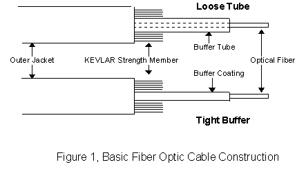
Figure 2 is a
drawing of the cross section details of a single and a two conductor fiber
optic cable as well as a more complex multi-fiber cable. Note that
the two conductor cable is similar to the common AC power line
electrical cable.
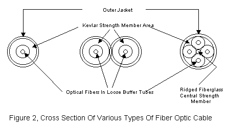
As
can be seen from the diagram, in all cases the fiber/buffer tube is first
enclosed in a layer of synthetic yarn such as Kevlar for strength.
An outer jacket of PVC or similar material is then extruded over
everything to protect the inside of the cable from the rigors of the
operating environment. In multi-fiber cables, an additional strength
member is also often added. While most fiber optic cables are
manufactured of totally non-conductive materials, there are some cable
that employ steel tape-wound outer jackets for rodent resistance (direct
burial types) or metallic strength members such as steel wire for aerial
(telephone pole) use. There are even fiber optic cables with
imbedded copper electrical conductors for transferring power to remote
electronic packages.
|
|
Whether loose-buffer or tight-buffer, the actual glass fiber used
in any fiber optic cable only comes in one of two basic types, multimode
fiber for use over short to moderate transmission distances (up to about
10 Km) and single-mode fiber for use over distances that are generally
greater than 10 Km. Communications grade multimode fiber normally
comes in two sizes, 50 micron core and 62.5 micron core, the latter being
the size most commonly available. The outer diameter of both is 125
microns and both use the same connector size. Single-mode fiber
comes in only one size, 8-10 microns for the core diameter and 125 microns
for the outer diameter. Connectors for single-mode fiber are not the
same as those designed for multimode fiber but can look the same as we
will soon discuss.
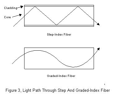
Figure 3 is a
drawing of the construction of two types of optical fiber, step index and
graded index.
Step index fiber has a core of ultra-pure
glass surrounded by a cladding layer of standard glass with a higher
refractive index. This causes light traveling within the fiber to
continually bounce between the walls of the core much like a ball
bouncing through a pipe. Graded index fiber on the other hand
operates by refracting (or bending) light continually toward the center of
the fiber like a long lens. In a graded index fiber the entire fiber
is made of ultra-pure glass. In both types of fiber however, the
light is effectively trapped and does not normally exit except at the far
end.
Losses in an optical
fiber are the result of absorption and impurities within the glass as well
as mechanical strains that bend the fiber at an angle that is so sharp
that light is actually able to leak out through the cladding
region. Losses are also dependent on the wavelength of the light
employed in a system since the degree of light absorption by glass varies
for different wavelengths. At 850 nanometers, the wavelength most
commonly used in short-range transmission systems, typical fiber has a
loss of 4 to 5 dB per kilometer of length. At 1300 nanometers this
loss drops to under 3 dB per kilometer and at 1550 nanometers, the loss is
a dB or so. The last two wavelengths are therefore obviously used
for longer transmission distances.
The losses described
above are independent of the frequency or data rate of the signals being
transmitted. There is another loss factor however that is frequency
(and wavelength) related and is due to the fact that light can have many
paths through the fiber. Figure 4 shows the mechanism of this
loss through step-index fiber.
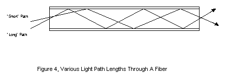
A light path
straighter through a fiber is shorter than a light path with maximum
bouncing. This means that for a fast rise-time pulse of light,
some paths will result in light reaching the end of the fiber sooner than
through other paths. This causes a smearing or spreading effect on
the output rise-time of the light pulse which limits the maximum speed of
light changes that the fiber will allow. Since data is usually
transmitted by pulses of light, this in essence limits the maximum data
rate of the fiber. The spreading effect for a fiber is expressed in
terms of MHz per kilometer. Standard 62.5 micron core multimode
fiber usually has a bandwidth limitation of 160 MHz per kilometer at 850
nanometers and 500 MHz per kilometer at 1300 nanometers due to its large
core size compared to the wavelength of the propagated light. Single
mode fiber, because of its very small 8 micron core diameter has a
bandwidth of thousands of MHz per kilometer at 1300 nanometers. For
most low frequency applications however, the loss of light due to
absorption will limit the transmission distance rather than the pulse
spreading effect. |
|
|
Since the tiny core of
an optical fiber is what transmits the actual light, it is imperative that
the fiber be properly aligned with emitters in transmitters,
photo-detectors in receivers and adjacent fibers in splices. This is
the function of the optical connector. Because of the small sizes of
fibers, the optical connector is usually a high precision device
with tolerances on the order of fractions of a thousandth of an inch.
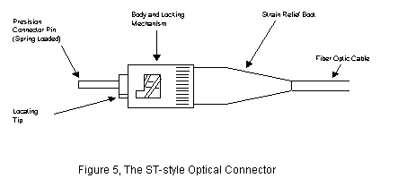
Although there are
many different styles available the most common optical cable connector in
current use is the ST type shown in figure 5. The connector
consists of a precision pin that houses the actual fiber, a spring-loaded
mechanism that presses the pin against a similar pin in a mating connector
(or electro-optic device) and a method of securing and strain-relieving
the outer jacket of the fiber optic cable. ST connectors are
available for both multimode and single-mode fibers. The main
difference between the two is the precision of the central pin.
Since this difference is not readily noticeable, care must be taken to use
the correct connector. While single-mode connectors will work
properly with multimode emitters and detectors, connectors intended for
use with multimode fiber such as the ST type will not work well (or at
all) in a single-mode system.
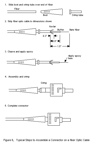
 The traditional
method for attaching optical connectors consists of first stripping the
jacket from the fiber cable with tools that are almost exact equivalents
of those used for electrical cable. Once this is done the strength
members are trimmed and inserted into various restraining grommets or
sleeves. For loose-tube fibers, the buffer tube is then removed
exposing the actual fiber. For tight-buffer fibers, the buffer
coating is removed with a precision stripping tool that looks like a small
wire stripper. The process, up to this point is still similar to
preparing copper wire. It is when the bare fiber is exposed
that the differences (compared to copper wire) occur. The stripped
fiber is now coated with a quick drying epoxy resin and inserted into a
precision hole or groove in the connector pin. Then the strain
relieving components are assembled and the basic connector is ready for
finishing. At this point the end of the bare fiber is protruding
from the front of the connector pin. The pin is placed in a special
tool that is then used to cleave or cut the tiny glass fiber flush with
the end of the pin. This takes a second or two. Next the
connector is placed into a small jig and run over two or three grades of
fine lapping film, the equivalent of ultra-fine sandpaper. This
completes the polishing of the fiber and the optical connector is ready
for use. The complete task, not including the 5 minutes of epoxy
drying time, takes anywhere from 5 to 10 minutes per connector depending
on the skill level of the person.
The traditional
method for attaching optical connectors consists of first stripping the
jacket from the fiber cable with tools that are almost exact equivalents
of those used for electrical cable. Once this is done the strength
members are trimmed and inserted into various restraining grommets or
sleeves. For loose-tube fibers, the buffer tube is then removed
exposing the actual fiber. For tight-buffer fibers, the buffer
coating is removed with a precision stripping tool that looks like a small
wire stripper. The process, up to this point is still similar to
preparing copper wire. It is when the bare fiber is exposed
that the differences (compared to copper wire) occur. The stripped
fiber is now coated with a quick drying epoxy resin and inserted into a
precision hole or groove in the connector pin. Then the strain
relieving components are assembled and the basic connector is ready for
finishing. At this point the end of the bare fiber is protruding
from the front of the connector pin. The pin is placed in a special
tool that is then used to cleave or cut the tiny glass fiber flush with
the end of the pin. This takes a second or two. Next the
connector is placed into a small jig and run over two or three grades of
fine lapping film, the equivalent of ultra-fine sandpaper. This
completes the polishing of the fiber and the optical connector is ready
for use. The complete task, not including the 5 minutes of epoxy
drying time, takes anywhere from 5 to 10 minutes per connector depending
on the skill level of the person.
Many people have
reservations about connectorizing fiber optic cable due to problems they
have heard about concerning the grinding and polishing of glass.
When one realizes that the grinding and polishing takes less than a
minute, and is done within a simple foolproof fixture, the mystery quickly
evaporates. In fact, assembling an ST style optical connector is, in
reality no more demanding a task than assembling an older style electrical
BNC. Once one is completely familiar with the process, (which takes
from 30 minutes to an hour to learn) the longest time interval involved in
the finishing process is waiting for the epoxy to cure.
Never-the-less the reservations continue. As a result, several
connector manufacturers manufacture so-called quick-crimp optical
connectors. These devices are installed with various mechanical
clamp arrangements and hot melt or instant bond adhesives (or, in some
cases no chemical adhesive at all). Some of these connectors are
even provided with a pre-polished length of optical fiber in the tip
thereby eliminating the finishing step altogether. Although these
are a bit easier to install, the original epoxy-polish method is really
not one that anyone should fear. Figure 6 shows the various
steps involved in installing conventional ST connectors.
Other optical
connectors that are available such as the SMA, SC and FCPC are similar in
principle in that they position the fiber in a close tolerance tip which
then mates with an equally precise device on the other end. They
really only differ from each other in the mechanical way that that
connectors mate to each other. In any event all optical connector
manufacturers provide detailed, easy to follow step-by-step installation
procedures for their respective connectors. |
|